G. Raymond Peacock

Temperatures.com, Inc.

Southampton, PA 18966

Abstract

A measurement of any kind has error. Carpenters know this well and they often measure twice before cutting once. Common tape measures have resolutions down to 1/16th of an inch, but errors of as much as 1/2″ are not uncommon. The best measurement is a statistical assessment of the result of repeated measurements. Measurements always have accompanying uncertainties that can be quantified and reported by measuring more than once.

This paper explains terminology and important statistics to help understand the basics of measurements, with an emphasis on infrared temperature, and the several key influences Nature and Man have on the process of dealing with them. If you have read the first modern standard on non-contact temperature sensor (radiation thermometer) measurement, ASTM E1256-15, you learned that even in a calibration lab it recommends the average of at least three measurements of blackbody source temperature in verifying an infrared thermometer’s calibration. Thus, measure thrice, report once is a more reliable approach to getting the best practical result.

Introduction

“Lies, damned lies, and statistics” is a phrase describing the persuasive power of numbers. But anytime one makes a measurement, of any parameter or variable, one is entering the world of numbers and statistics. To try to avoid them is not only impossible, it is foolish.

If you report temperatures or temperature difference, better take care to do it correctly.

Why are statistics involved? It’s like the old carpenter’s adage: “Measure twice, cut once”. Statistics is the way to understand and correct results for measurement errors rather than to pretend they don’t exist. Every measurement has an error and it takes at least three tries to get some idea of its size. So the carpenter’s rule should, in truth, state: “Measure at least thrice before cutting once”.

Thermographers, Meteorologists and Metrologists all face the same issues with measurements in reporting Temperatures, Weather properties and Calibrations, respectively. They all do, or are well-advised to, use statistics in a professional, but not difficult, way. However, this is getting ahead of the story I want to tell; the one about how you get to the point of using statistics, and the why and how.

“Infrared Camera Accuracy and Uncertainty” is the title of a recent online article by FLIR Systems (http://www.flir.eu/science/blog/details/?ID=74935) in an effort to help users better understand some of the terminology around measurement errors, but it didn’t delve very far into the statistics beyond a few formulae.

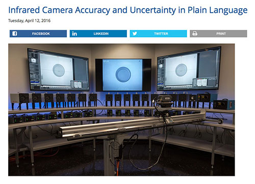
My news website reported on it along with some additional resources at http://www.tempsensornews.com/generic-temp-sensors/infrared-camera-accuracy-and- uncertainty/

The original article is on the European FLIR Blog at: http://www.flir.eu/science/blog/details/?ID=74935.

Looking back, I realize that 14 years ago, I attempted a similar explanation at the 2003 IR/INFO (Reference 1). It covered more ground than the FLIR article, but tried to do too much, I now realize. In my opinion, neither article is really simple. The topic is complex.

As a former mentor of mine used to say: “If you break down a complicated subject into basic components and explain those well, then things get easier to understand.” So, here goes another attempt to really make this very important topic easier to understand by considering first some fundamental pieces.

Some Fundamentals: A Review

Laboratory measurements quantifying the calibration uncertainty of a thermal imager involve pointing the camera at a calibrated, uniform blackbody source and recording/reading the output temperatures over a period of time. The test is repeated at different source temperatures and the differences in measured versus standard temperatures are measured, errors reported and lab uncertainty calculated for each calibration point or for the entire series. There are various methods.

Uncertainty is a measure of the dispersion of the errors of the individual measurements. Lab calibration personnel follow prescribed standards and procedures to produce a calibration report or match a lab requirement for calibration uncertainty. To emphasize: individual measurements have errors and the dispersion of the errors is quantified as the measurement uncertainty, or the likely region in which the true measured temperature lies. This is true in a calibration lab and in the “Real World”, but it is more difficult in the “Real World” as I will explain.

The terminology properly used states that the uncertainty in a measurement result is a numerical value plus or minus some variation for a set of confidence limits. A typical uncertainty statement, say for a calibration certificate would look like:

The Calibration Uncertainty of this device at a temperature of 212 Degs F is +/- 1 Deg F with a confidence limit of 95%.

This may sound foreign to some, so here are a few terms that are worth describing in more detail before going further.

First, Accuracy: Accuracy is a term that describes how closely a measuring device comes to a standard, but not in numbers. So, someone who states that the accuracy of their measurement device is, say, 2% or 2 degrees, is not being precise, to be precise. They mix apples and oranges.

“Accuracy” is a qualitative or descriptive term, expressed in words, like: “That instrument is in the 10 Degrees F accuracy category”.

“Error” is the amount by which an individual measurement departs from some norm. It is quantitative. It is expressed numerically, like: The error at 100 Degrees F is +3 Degrees.

“Uncertainty” is quantitative and is defined as follows (Reference 1): “A parameter associated with the result of a measurement that characterizes the dispersion of the values that could reasonably be attributed to the measurand (VIM Ref 4); the range assigned to a measurement result that describes, within a defined level of confidence, the limits expected to contain the true measurement result. Uncertainty is a quantified expression of measurement reliability.”

Uncertainty is a property of each measurement, a measure of the dispersion of the errors of an instrument under certain conditions. Errors are variable and most easily measured in the calibration or standards laboratory, traceable to the International Temperature Scale of 1990 (ITS-90), or a later standard. Every temperature value on that scale has established uncertainty values also. One can learn more about ITS-90 details by visiting the website of the International Bureau of Weights and Measures, called BIPM, at http://bipm.org.

Measurement errors are more difficult to measure in the field, since one has very few standards with which to compare the results reported by your device in each measurement. In addition, there are many factors that can introduce both internal and external errors during the use of a thermal imager. So, “Real World” measurement uncertainty is not as easy to define and quantify as that of the calibration, or metrological, uncertainty. Determining both requires some relatively simple statistical calculations.

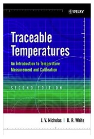
The book, “Traceable Temperatures” has been my “Go To” reference since the early 1990’s when it was first published (Reference 2). I highly recommend the latest Edition of this book for anyone who is serious about measuring temperature by any means, contact or non- contact. It helps greatly in understanding the properties of many different types of temperature sensors, including Radiation Thermometry. Plus, it has a great introduction to both temperature and uncertainty in measurement in measuring it.

There are, in fact, two fundamentally different uncertainties that affect a measuring device’s results.

They are: Calibration Uncertainty and the Application Uncertainty.

The overall measuring uncertainty that a Thermographer in the field must deal with is their combined effects. The statistically correct method of combining uncertainties is described nicely in the FLIR article as the Root Sum of the Squares (RSS) combination of errors, or,

Total Uncertainty squared = Calibration (C) Uncertainty squared + Application (A) Uncertainty squared

Or Total U^2 = CU^2 + AU^2

Considering that an Application uncertainty has two components, Internal (I) and External (E), the above equation has at least an additional term:

Total U^2 = CU^2 + AU^2 = CU^2 + IU^2 + ExU^2

There are many examples of the methods used to describe measurement uncertainty; some that I know are listed in the References section at the end of this paper.

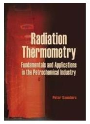
One very useful reference is the free online white paper from Beamex entitled Calibration uncertainty for non-mathematicians (Reference 3). Yet another, a paid download at the SPIE Digital Library, is an excellent little book by Dr. Peter Saunders of New Zealand’s National Measurement Institute, Radiation Thermometry, Fundamentals and Applications in the Petrochemical Industry (Reference 4). Not only is this a very thorough coverage of the principles of Radiation Thermometry, the same technology that a thermal imaging camera uses to produce temperature readings, it provides a series of worked uncertainty examples in radiation thermometry field measurements.

So, why and how do we get to “Measurement Uncertainty”?

And, furthermore, what is it really and why haven’t we heard about it before?

The two basic calculations to quantify the dispersion of a series of measurements in the field, and calculate the uncertainty, are the Mean (M) of the measurements followed by calculation of their Standard Deviation (SD).

The mean is the sum of the individual measurements divided by the number of measurements.

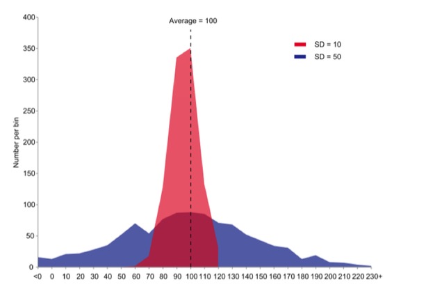
Graph by JRBrown – Own work, Public Domain,
https://commons.wikimedia.org/w/index.php?curid=10777712

But the mean is not enough to quantify a sample set of measurements. The graph above shows two sets of data with the same mean value, but widely different spread, or variation, in the data. The standard deviation is the square root of the variance of the measurements and, in turn, the variance is the average of the squared differences from the Mean.

The basic uncertainty for a random, or Normal distribution of the results is expressed as U = +/- SD. This yields the uncertainty with a confidence limit of 68% for a very large set of measurement data points. In such a case the true value, within a confidence of 68%, lies between the average value and plus or minus one standard deviation.

The expanded uncertainty of the results is expressed as U = +/- k*SD, where k is the coverage factor of 1, 2, or 3. The k values stand for confidence limits of: 1 for 68%, 2 for 95% and 4 for 99.7%, for a random or Normal distribution of the measurements.

Then, once the Application Uncertainty is determined, it must be combined, as described above, with the Calibration Uncertainty to correctly calculate the overall uncertainty. The key to doing it correctly is that both the major uncertainty components are at the same level of confidence. That latter requirement makes it extremely difficult to calculate – with some certainty – if the manufacturer’s literature, or supplied calibration certificate, does not specify the calibration uncertainty of its products.

The international effort to improve manufacturing product Quality resulted in ISO 2000 standards. It also resulted in the development of The Guide for the Use of Terminology in Measurements (GUM) (Reference 5) and the ISO 17025 standards a little later that have been adopted worldwide by most Standards authorities, including ASTM. In the past 25 years, they have become the international and national norms for reporting and describing measurement results in science and technology.

This terminology is probably new to most readers, but it is the terminology that those who are serious about measurement and truly understand it, use.

The first error is described in the Traceable Calibration Certificate for the device, usually provided by the device supplier, and often beyond the capability of the user. Although, it is not too difficult to periodically verify that a device has not shifted in calibration beyond the maker’s specification.

The Application, or Use Error is another story. That’s where the “Measure Thrice” (at least) comes in and where one has to work a little harder to quantify the dispersion of measurement results. Measuring a very large number of data points is not easy in the field, but one or two are not enough, especially if one hopes to produce reliable results.

Application Uncertainty: Measuring Thrice (or more)

The best way to find the measurement uncertainty in an application is to take a series of measurements, if possible and required, on one or more locations on the object area of interest. If you stick with three measurements, you add the three results and divide by 3 to get the average result. Note, too, that if you take more measurements, the SD of the results gets smaller by the square root of the number of measurements.

You need to calculate the measurements’ standard deviation, as described above. This alternately can be done by using a basic scientific calculator; all have built-in features for both quantities. So too, do spreadsheets such as MS Excel and Apple Numbers.

There are some interesting features in the use of statistics in measurement that are worth noting.

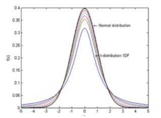
First, the more measurements that you take, most times, helps reduce your standard deviation, since the coverage factors described above are for a normal distribution of results about the mean value. See the outer curve on the graph here.

Then, the assumption that most make, is that the variations in measurement results are based on a randomness of the temperature variations we measure.

NOTE: If you do not see variations in repeated measurements of your objects’ temperatures, then your measurement device is insensitive to them and you have the equivalent situation of using a yardstick to measure the diameter of a thread. In such a case you have no idea of its actual diameter or the variations in it.

If you do see measurable variations in the temperature and they are within your measuring temperature limits, then you have a correct starting point. Your measured temperatures are what statisticians call samples of a population with n elements or values. If the distribution of the values are random, then your samples’ parameters of mean and SD values will be related to the mean and SD of the population.

This problem has been studied many times in the past by many mathematicians. It depends on the number of degrees of freedom in a given measurement, or the number of measurements. If there are n measurements, there are n-1 degrees of freedom.

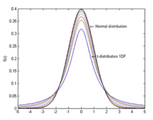
This is where the details begin to get complicated and one has to get into more detailed statistics and something called the student’s t-distribution and statistics. Student’s t- distribution – plots of 1, 2, 3, 4, 5,10, 20, 50 and an Infinite Degrees of Freedom (or 2, 3, 4, 5, 11, 21, 51) and an infinite number of samples, or the Normal Distribution (limiting distribution)

The t-distribution plays a role in a number of widely used statistical analyses, but here in this graph, one can see the differences between the Student’s t-distribution and the Normal, or random, distribution.

The same graph used above and shown here again shows the probability that the standard deviation of a sample will fall within the
limits shown by the curve. The inner curves are for “small” samples, typically less than 50. Above 50 the Normal distribution is implied since it is so close to it.

The easiest way to find the probability associated with less than 51 samples is to use the t Distribution Calculator, a free tool provided by Stat Trek online at http://stattrek.com/online-calculator/t-distribution.aspx.

The consequence of all this statistics talk is to show that taking more samples (making more measurements) improved the calculation of the Uncertainty by reducing the size of the standard deviation times the coverage factor for a particular confidence interval. It shows that in the case of three measurements, the k factors to be used in the above formulas for calculating the uncertainties change the coverage factors as follows:

• For 68% confidence intervals, 2 samples will have a SD multiplier of 1.8, for 3 samples, it’s about 1.3, 5 samples it’s 1.1 and 50 samples it’s 1.0.
• For 95% confidence intervals, 2 samples will have a SD multiplier of 12.7, for 3 samples, it’s about 4.3, for 5 samples it’s 2.8 and for 50 samples it’s 2.0.
• For 99.5% confidence intervals, 2 samples will have a SD multiplier of 127.3, for 3 samples, it’s 14.1, for 5 samples, it’s 5.6 and for 50 samples, it’s 3.0.
•  

Bottom Line: measuring thrice over twice is a big improvement in reducing the amount of measurement uncertainty when one seeks the best confidence in the results. Measuring even more samples reduces Uncertainties even more.

To Recap:

1. Multiple measurements in the field are required to determine temperature and temperature difference averages and variation, with confidence limits, so as to be able to state the results of your measurements in statistically correct terms.
2. A full statement of results must include the calibration uncertainty using the same confidence limits.
3. It’s not very difficult to do the above, but it takes some understanding and care.

Summary

The proper professional way to report measured temperatures is to use the technical terms and calculations agreed upon internationally among measurement professionals of all nations and their agreed vocabulary. It has been written about and widely publicized for more than 15 years. There are numerous free and paid resources to help thermographers learn how to use them.

In this paper I have only discussed what are called Type A Uncertainties. There are also Type B and then some way to combine them. Suffice it to say, the dominant problem in the field one is usually determining are Type A ones.

Additional resources to learn more about Type B Uncertainties and the Student’s t- distribution table are contained in the References Section.

References

1. Confidence Limits in Temperature Measurements, G. Raymond Peacock, IR/INFO 2003
2. Temperatures (An Introduction to Temperatures Measurement and Calibration), Second Edition, J. V. Nicholas & D. R. White, John Wiley & Sons, LTD, 2001
3. Calibration uncertainty for non-mathematicians, Free download at: http://resources.beamex.com/calibration-uncertainty-for-non-mathematicians. (This online white paper discusses the basics of uncertainty in measurement and calibration. The paper is designed for people who are not mathematicians or metrology experts, but rather to people who are planning and making the practical measurements and calibrations in industrial applications.)
4. Radiation Thermometry, Fundamentals and Applications in the Petrochemical Industry, Peter Saunders, SPIE (tutorial texts in optical engineering) 2007. (Available online at http://spie.org/Publications/Book/741687)
5. GUM: Guide to the Expression of Uncertainty in Measurement is a free download online at: http://www.bipm.org/en/publications/guides/gum.html
6. NIST/SEMATECH e-Handbook of Statistical Methods, https://www.nist.gov/programs-projects/nistsematech-engineering-statistics- handbook, (A free Web-based book written to help scientists and engineers incorporate statistical methods into their work as efficiently as possible.) NIST (USA)
7. Introduction to Measurement Uncertainty, NPL e-Learning Program is a paid set of online videos (intro video is free) at: http://www.npl.co.uk/commercial- services/products-and-services/training/e-learning/introduction-to-uncertainty/
8. Essentials of expressing measurement uncertainty, http://physics.nist.gov/cuu/Uncertainty/index.html, NIST (USA).
9. NPL’s Beginner’s Guide to Temperature, http://www.npl.co.uk/educate-explore/factsheets/temperature/temperature-(poster), National Physical Laboratory, Last Updated: 7 Aug 2015
10. The kelvin, https://www.youtube.com/watch,v=PzoxxNefCUw&index=3&list=PLBB61840785E D0B1D, and http://www.npl.co.uk/reference/measurement-units/si-base-units/the- kelvin, National Physical Laboratory
11. VIM: International Vocabulary of Metrology – Basic and General Concepts and Associated Terms (VIM 3rd edition) – JCGM 200:2012 (JCGM 200:2008 with minor corrections) http://www.bipm.org/utils/common/documents/jcgm/JCGM_200_2012.pdf;
12. Calibration and R&R Practices for Reliable Temperature Measurements, G. Raymond Peacock, IR/INFO 2005
13. The Role of Standards & Calibration in IR Thermography, G. Raymond Peacock, IR/INFO 2011
14. Procedure for calibration and verification of the main characteristics of thermographic instruments- (Confirmed 2008-10-31) is online as a free downloadable pdf document. (www.oiml.org/publications/R/R141-e08.pdf)