
Reliability Engineer & Condition Monitoring Specialist
Perth, Western Australia, Australia
Ph: +61 46 744 3834
In the field of IRT, we learn that Total Radiosity is a combination of Emissivity, Reflectivity, and Transmissivity (E+R+T=1). It is a concept that takes time to get your head around, but one that is essential to master on the road to becoming an effective thermographer.
While conducting a thermal imaging survey as part of a condition monitoring program in a Data Center, I encountered a situation that gave me an opportunity to further understand the effect of reflected temperature on total radiosity.
I was scanning a run of electrical busduct that was lightly loaded (21% of rated load). For good thermal contrast, the minimum recommended load is 40%. However, this run would not increase in load for several months, and therefore had to be captured under current conditions at this time to ensure compliance for maintenance procedures.
With poor thermal contrast, I was struggling to maintain focus with the telephoto lens attached to the imager. My first step to rectify this was to switch from High Contrast (my palette of choice) to Greyscale. This was a tip passed on from my IRT instructor, which is another good reason why training is paramount. Practitioners with a wealth of experience are happy to pass their knowledge on, so thank you!
The change of palette helped a lot, but my auto temperature range settings were also hampering me. I find that the auto function usually increases efficiency when surveying a large electrical room that houses equipment at different loads, but in this instance the auto range was causing the image to wash out and it needed to be manually tuned.
I set the background temp in the IR camera to 24 C, which is typically a good starting point for this location. The first 4 x inspection points revealed max temperatures ranging between 30 – 32 C, which established my baseline. Any significant variance above this would be potentially anomalous. So, after playing around with the tuning, I found the range which provided best thermal contrast and focus was 18 – 32 C.
Moving along the run (14 points of inspection total), I was satisfied with the thermograms given the conditions. Then, as I transitioned to the next to last point, a red pattern bled into the image. The camera was detecting a temperature on the target that exceeded the range I had manually set and, as it is designed to do, applied an isotherm to highlight those areas for the operator’s attention.
Red alert – Had I just found an issue? I steadied my position and allowed the camera to stabilize. The pattern adjusted as my position shifted, so I quickly realized the isotherm was indicating the reflective temperature gain from the roof of the transformer housing approximately three feet below.
The thermal energy was rising and reflecting off the higher reflective (lower emissive) components of the joint pack, even down to the granular differences within the paint coating itself, indicated by the sparse red spotting. This discovery was made possible because the busduct was uniformly coated in a substance that had an accepted emissivity of 0.95, so anything below that was going to be more reflective in comparison.
It was educational to actually “see” how reflective temperature impacts a target. Plus, it also had the added value of making the survey a little more interesting!
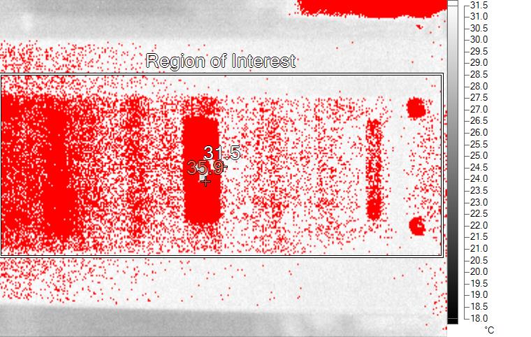
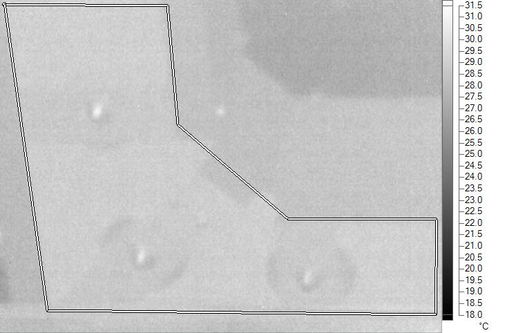
The white center point marker on the highly emissive surface shows the apparent temperature measurement (31.5 C) and the red floating marker on the highly reflective surface shows the max temp measurement (35.9 C). The difference between these two measurements (4.4 C) represents the reflective temperature gain. In the thermogram below, the preceding inspection point on the run has a similar apparent surface temp but shows no red pattern with the same tuning applied. This is because that point is out of range from any intense reflective temperature sources like the TX.
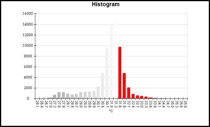
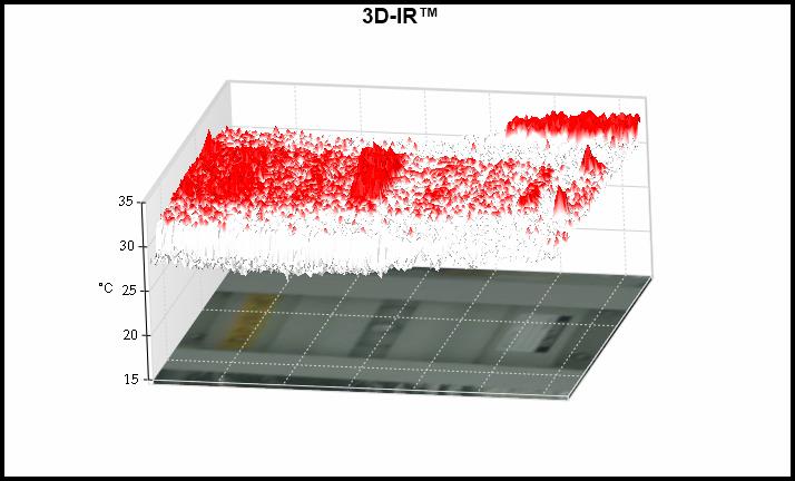
The Histogram clearly delineates the reflective portion from total radiosity in the distribution, while the surface level reflected temperature is enhanced in the 3D-IR model, which I think aids visual understanding.
Conclusion
Reflective temperature changes from target to target, so it is important to account for it and understand its effect on total radiosity. Even in a temperature controlled environment such as this, a one time set and forget background temperature could lead to a false positive if not considered in the analysis.
It is worth remembering to always understand the equipment being surveyed, what technique can get the best result from the IR camera, and use your training to understand what the thermographic data is telling us.
From a design for reliability perspective, thumbs up to the manufacturer for incorporating the paint coating into the evolution of the design. It enables us thermographers to capture a more definitive picture of the equipment’s current condition.
I’ll leave you with a temp-lapseof the reflection bleeding into the image as the temperature range is dialed in.
